Timeseries Partitioning in Compactor
- Author: @roystchiang
- Reviewers:
- Date: August 2022
- Status: Proposed
Timeseries Partitioning in Compactor
Introduction
The compactor is a crucial component in Cortex responsible for deduplication of replicated data, and merging blocks across multiple time intervals together. This proposal will not go into great depth with why the compactor is necessary, but aims to focus on how to scale the compactor as a tenant grows within a Cortex cluster.
Problem and Requirements
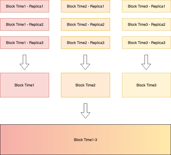
Cortex introduced horizontally scaling compactor which allows multiple compactors to compact blocks for a single tenant, sharded by time interval. The compactor is capable of compacting multiple smaller blocks into a larger block, to reduce the duplicated information in index. The following is an illustration of how the shuffle sharding compactor works, where each arrow represents a single compaction that can be carried out independently.
However, if the tenant is sending unique timeseries, the compaction process does not help with reducing the index size. Furthermore, this scaling of parallelism by time interval is not sufficient for a tenant with hundreds of millions of timeseries, as more timeseries means longer compaction time.
Currently, the compactor is bounded by the 64GB index size, and having a compaction that takes days to complete simply is not sustainable. This time includes the time to download the blocks, merging of the timeseries, writing to disk, and finally uploading to object storage.
The compactor is able to compact up to 400M timeseries within 12 hours, and will fail with the error of index exceeding 64GB. Depending on the number of labels and the size of labels, one might reach the 64GB limit sooner. We need a solution that is capable of:
- handling the 64GB index limit
- reducing the overall compaction time
- downloading the data in smaller batches
- reducing the time required to compact
Design
A reminder of what a Prometheus TSDB is composed of: an index and chunks. An index is a mapping of timeseries to the chunks, so we can do a direct lookup in the chunks. Each timeseries is effectively a set of labels, mapped to a list of <timestamp, value> pair. This proposal focuses on partitioning of the timeseries.
Partitioning strategy
The compactor will compact a overlapping time-range into multiple sub-blocks, instead of a single block. Cortex can determine which partition a single timeseries should go into by applying a hash to the timeseries label, and taking the modulo of the hash by the number of partition. This guarantees that with same number of partition, the same timeseries will go into the same partition.
partitionId = Hash(timeseries label) % number of partition
The number of partition will be determined automatically, via a configured multiplier. This multiplier factor allows us to group just a subset of the blocks together to achieve the same deduplication factor as having all the blocks. Using a multiplier of 2 as an example, we can do grouping for partition of 2, 4 and 8. We’ll build on the actual number of partition determination in a later section.
Determining overlapping blocks
In order to reduce the amount of time spent downloading blocks, and iterating through the index to filter out unrelated timeseries, we can do smart grouping of the blocks.
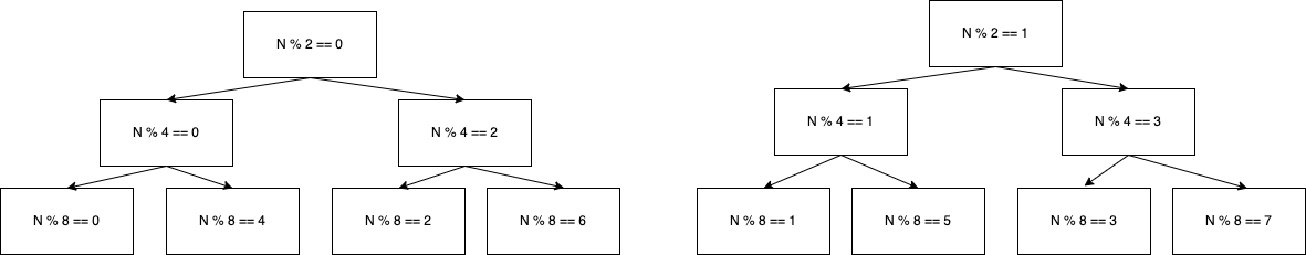
Given that we are always multiplying the number of partition by the multiplier factor, we can deduce from the modulo which partition could contain overlapping result
Given a hash N, if N % 8 == 7, then N % 4 must be 3
Given a hash N, if N % 8 == 3, then N % 4 must be 3
Given a hash N, if N % 8 == 4, then N % 4 must be 0
Given a hash N, if N % 8 == 0, then N % 4 must be 0
Hence it is safe to group blocks with N % 8 == 7 with N % 8 == 3 together with N % 4 == 3 together, and we are sure that other blocks won’t contain the same timeseries. We also know that if N % 8 == 0, then we don’t need to download blocks where N % 4 == 1 or N % 4 == 2
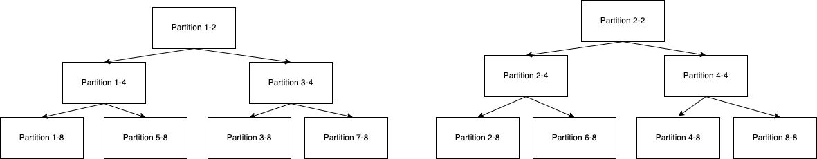
Given partition count and partition id, we can immediately find out which blocks are required. Using the above modulo example, we get the following partitiong mapping.
Planning the compaction
The shuffle sharding compactor introduced additional logic to group blocks by distinct time intervals. It can also sum up the sizes of all indices to determine how many shards are required in total. Using the above example again, and assuming that each block has an index of 30GB, the sum is 30GB * 14 = 420GB, which needs to be at least 7, since maximum index size is 64GB. Using the multiplier factor, it will be rounded up to 8.
Now the planner knows the resulting compaction will have 8 partitions, it can start planning out which groups of blocks can go into a single compaction group. Given that we need 8 partitions in total, the planner will go through the process above to find out what blocks are necessary. Using the above example again, but we have distinct time intervals, T1, T2, and T3. T1 has 2 partitions, T2 has 4 partitions, and T3 has 8 partitions, and we want to produce T1-T3 blocks
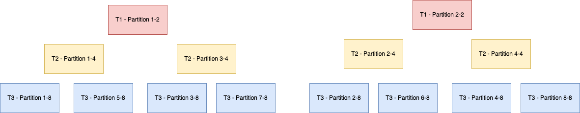
Compaction Group 1-8
T1 - Partition 1-2
T2 - Partition 1-4
T3 - Partition 1-8

Compaction Group 2-8
T1 - Partition 2-2
T2 - Partition 2-4
T3 - Partition 2-8

Compaction Group 3-8
T1 - Partition 1-2
T2 - Parittion 3-4
T3 - Partition 3-8

Compaction Group 4-8
T1 - Partition 2-2
T2 - Partition 4-4
T3 - Partition 4-8

Compaction Group 5-8
T1 - Partition 1-2
T2 - Partition 1-4
T3 - Partition 5-8

Compaction Group 6-8
T1 - Partition 2-2
T2 - Partition 2-4
T3 - Partition 6-8

Compaction Group 7-8
T1 - Partition 1-2
T2 - Partition 3-4
T3 - Partition 7-8

Compaction Group 8-8
T1 - Partition 2-2
T2 - Partition 4-4
T3 - Partition 8-8
T1 - Partition 1-2 is used in multiple compaction groups, and the following section will describe how the compaction avoids duplicate timeseries in the resulting blocks
Compaction
Now that the planner has produced a compaction plan for the T1-T3 compaction groups, the compactor can start downloading the necessary blocks. Using compaction group 1-8 from above as example.
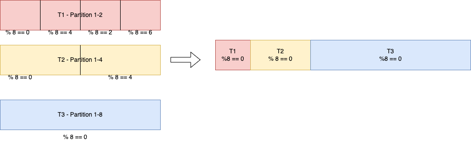 T1 - Partition 1-2 was created with hash % 2 == 0, and in order to avoid having duplication information in blocks produced by compaction group 3-8, compaction group 5-8, and compaction group 7-8, we need apply the filter the
 %8 == 0 hash, as that’s the hash of the highest partition count.
Compaction Workflow
- Compactor initializes Grouper and Planner.
- Compactor retrieves block’s meta.json and call Grouper to group blocks for compaction.
- Grouper generates partitioned compaction groups:
- Grouper groups source blocks into unpartitioned groups.
- For each unpartitioned group:
- Generates partitioned compaction group ID which is hash of min and max time of result block.
- If the ID exists under the tenant directory in block storage, continue on next unpartitioned group.
- Calculates number of partitions. Number of partitions indicates how many partitions one unpartitioned group would be partitioned into based on the total size of indices and number of time series from each source blocks in the unpartitioned group.
- Assign source blocks into each partition with partition ID (value is in range from 0 to number_of_partitions - 1). Note that one source block could be used in multiple partitions (explanation in Planning the compaction and Compaction). So multiple partition ID could be assigned to same source block. Check more partitioning examples in Compaction Partitioning Examples
- Generates partitioned compaction group that indicates which partition ID each blocks got assigned.
- Partitioned compaction group information would be stored in block storage under the tenant directory it belongs to and the stored file can be picked up by cleaner later. Partitioned compaction group information contains partitioned compaction group ID, number of partitions, list of partitions which has partition ID and list of source blocks.
- Store partitioned compaction group ID in block storage under each blocks’ directory that are used by the generated partitioned compaction group.
- Grouper returns partitioned compaction groups to Compactor. Each returned group would have partition ID, number of partitions, and list of source blocks in memory.
- Compactor iterates over each partitioned compaction group. For each iteration, calls Planner to make sure the group is ready for compaction.
- Planner collects partitioned compaction group which is ready for compaction.
- For each partitions in the group and for each blocks in the partition:
- Make sure all source blocks fit within the time range of the group.
- Make sure each source block with assigned partition IDs is currently not used by another ongoing compaction. This could utilize visit marker file that is introduced in #4805 by expanding it for each partition ID of the source block.
- If all blocks in the partition are ready to be compacted,
- mark status of those blocks with assigned partition ID as
pending. - The status information of each partition ID would be stored in block storage under the corresponding block directory in order for cleaner to pick it up later.
- mark status of those blocks with assigned partition ID as
- If not all blocks in the partition are ready, continue on next partition
- For each partitions in the group and for each blocks in the partition:
- Return all ready partitions to Compactor.
- Compactor starts compacting partitioned blocks. Once compaction completed, Compactor would mark status of all blocks along with assigned partition ID in the group as
completed. Compactor should use partitioned compaction group ID to retrieve partitioned compaction group information from block storage to get all partition IDs assigned to each block. Then, retrieve status information of each partition ID this assigned to block under current block directory in block storage. If all assigned partition ID of the block have status set tocompleted, upload deletion marker for this block. Otherwise, no deletion marker would be uploaded.
Clean up Workflow
Cleaner would periodically check any tenants having deletion marker. If there is a deletion marker for the tenant, Cleaner should remove all blocks and then clean up other files including partitioned group information files after tenant clean up delay. If there is no deletion marker for tenant, Clean should scan any source blocks having a deletion marker. If there is a deletion marker for the block, Cleaner should delete it.
Performance
Currently a 400M timeseries takes 12 hours to compact, without taking block download into consideration. If we have a partition count of 2, we can reduce this down to 6 hours, and a partition count of 10 is 3 hours. The scaling is not linear, and I’m still attempting to find out why. The initial result is promising enough to continue though.
Alternatives Considered
Dynamic Number of Partition
We can also increase/decrease the number of partition without needing the multiplier factor. However, if a tenant is sending highly varying number of timeseries or label size, the index size can be very different, resulting in highly dynamic number of partitions. To perform deduplication, we’ll end up having to download all the sub-blocks, and it can be inefficient as less parallelization can be done, and we will spend more time downloading all the unnecessary blocks.
Consistent Hashing
Jump consistent hash, rendezvous hashing, and other consistent hashing are great algorithms to avoid reshuffling of data when introducing/removing partitions on the fly. However, it does not bring much of a benefit when determining which partition contains the same timeseries, which we need to deduplication of index.
Partition by metric name
It is likely that when a query comes, a tenant is interested in an aggregation of a single metric, across all label names. The compactor can partition by metric name, so that all timeseries with the same name will go into the same block. However, this can result in very uneven partitioning.
Architecture
Planning
The shuffle partitioning compactor introduced a planner logic, which we can extend on. This planner is responsible for grouping the blocks together by time interval, in order to compact blocks in parallel. The grouper can also determine the number of partition by looking at the sum of index file sizes. In addition, it can also do the grouping of the sub-blocks together, so we can achieve even higher parallelism.
Clean up
Cortex compactor cleans up obsolete source blocks by looking at a deletion marker. The current architecture does not have the problem of having a single source block involved in multiple compaction. However, this proposal is able to achieve higher parallelism than before, hence it is possible that a source block is involved multiple times. Changes needs to be made on the compactor regarding how many plans a particular blocked is involved in, and determining when a block is safe to be deleted.
Changes Required in Dependencies
Partitioning during compaction time
Prometheus exposes the possibility to pass in a custom mergeFunc. This allows us to plug in the custom partitioning strategy. However, the mergeFunc is only called when the timeseries is successfully replicated to at least 3 replicas, meaning that we’ll produce duplicate timeseries across blocks if the data is only replicated once. To work around the issue, we can propose Prometheus to allow the configuration of the MergeChunkSeriesSet.
Source block checking
Cortex uses Thanos’s compactor logic, and it has a check to make sure the source blocks of the input blocks do not overlap. Meaning that if BlockA is produced from BlockY, and BlockB is also produced from BlockY, it will halt. This is not desirable for us, since partitioning by timeseries means the same source blocks will produce multiple blocks. Reason for having this check in Thanos is supposed to prevent having duplicate chunks, but the change was introduced without knowing whether it will actually help. We’ll need to introduce a change in Thanos to disable this check, or start using Thanos compactor as a library instead of a closed box.
Work Plan
- Performance test the impact on query of having multiple blocks
- Get real data on the efficiency of modulo operator for partitioning
- Get the necessary changes in Prometheus approved and merged
- Get the necessary changes in Thanos approved and merged
- Implement the number of partition determination in group
- Implement the grouper logic in Cortex
- Implement the clean up logic in Cortex
- Implement the partitioning strategy in Cortex, passed to Prometheus
- Produce the partitioned blocks
Appendix
Risks
- Is taking the modulo of the hash sufficient to produce a good distribution of partitions?
- What’s the effect of having too many blocks for the same time range?
Frequently Asked Questions
- Are we able to decrease the number of partition?
- Using partitions of 2, and 4, and 8 as example
T1 partition 1 - Hash(timeseries label) % 2 == 0
T1 partition 2 - Hash(timeseries label) % 2 == 1

T2 partition 1 - Hash(timeseries label) % 4 == 0
T2 partition 2 - Hash(timeseries label) % 4 == 1
T2 partition 3 - Hash(timeseries label) % 4 == 2
T2 partition 4 - Hash(timeseries label) % 4 == 3

T3 partition 1 - Hash(timeseries label) % 8 == 0
T3 partition 2 - Hash(timeseries label) % 8 == 1
T3 partition 3 - Hash(timeseries label) % 8 == 2
T3 partition 4 - Hash(timeseries label) % 8 == 3
T3 partition 5 - Hash(timeseries label) % 8 == 4
T3 partition 6 - Hash(timeseries label) % 8 == 5
T3 partition 7 - Hash(timeseries label) % 8 == 6
T3 partition 8 - Hash(timeseries label) % 8 == 7

We are free to produce a resulting timerange T1-T3, without
having to download all 14 blocks in a single compactor

If T1-T3 can fit inside 4 partitions, we can do the following grouping

T1 partition 1 - Hash(timeseries label) % 2 == 0 && % 4 == 0
T2 partition 1 - Hash(timeseries label) % 4 == 0 &&
T3 partition 1 - Hash(timeseries label) % 8 == 0
T3 partition 5 - Hash(timeseries label) % 8 == 4

T1 partition 2 - Hash(timeseries label) % 2 == 1 && % 4 == 01
T2 partition 2 - Hash(timeseries label) % 4 == 1
T3 partition 2 - Hash(timeseries label) % 8 == 1
T3 partition 7 - Hash(timeseries label) % 8 == 5

T1 partition 1 - Hash(timeseries label) % 2 == 0 && % 4 == 2
T2 partition 3 - Hash(timeseries label) % 4 == 2
T3 partition 3 - Hash(timeseries label) % 8 == 2
T3 partition 7 - Hash(timeseries label) % 8 == 6

T1 partition 2 - Hash(timeseries label) % 2 == 1 && % 4 == 3
T2 partition 4 - Hash(timeseries label) % 4 == 3
T3 partition 4 - Hash(timeseries label) % 8 == 3
T3 partition 8 - Hash(timeseries label) % 8 == 7

If T1-T3 can fit inside 16 partitions, we can do the same grouping, and hash on top

T1 partition 1 - Hash(timeseries label) % 2 == 0 && % 8 == 0
T2 partition 1 - Hash(timeseries label) % 4 == 0 && % 8 == 0
T3 partition 1 - Hash(timeseries label) % 8 == 0

T1 partition 2 - Hash(timeseries label) % 2 == 1  && % 8 == 1
T2 partition 2 - Hash(timeseries label) % 4 == 1  && % 8 == 1
T3 partition 2 - Hash(timeseries label) % 8 == 1

T1 partition 1 - Hash(timeseries label) % 2 == 0 && % 8 == 2
T2 partition 3 - Hash(timeseries label) % 4 == 2 && % 8 == 2
T3 partition 3 - Hash(timeseries label) % 8 == 2

T1 partition 2 - Hash(timeseries label) % 2 == 1 && % 8 == 3
T2 partition 4 - Hash(timeseries label) % 4 == 3 && % 8 == 3
T3 partition 4 - Hash(timeseries label) % 8 == 3

T1 partition 1 - Hash(timeseries label) % 2 == 0 && % 8 == 4
T2 partition 1 - Hash(timeseries label) % 4 == 0 && % 8 == 4
T3 partition 5 - Hash(timeseries label) % 8 == 4

T1 partition 2 - Hash(timeseries label) % 2 == 1 && % 8 == 5
T2 partition 2 - Hash(timeseries label) % 4 == 1 && % 8 == 5
T3 partition 6 - Hash(timeseries label) % 8 == 5

T1 partition 1 - Hash(timeseries label) % 2 == 0 &&  % 8 == 6
T2 partition 3 - Hash(timeseries label) % 4 == 2 &&  % 8 == 6
T3 partition 7 - Hash(timeseries label) % 8 == 6

T1 partition 2 - Hash(timeseries label) % 2 == 1 && % 8 == 7
T2 partition 4 - Hash(timeseries label) % 4 == 3 && % 8 == 7
T3 partition 8 - Hash(timeseries label) % 8 == 7
Compaction Partitioning Examples
Scenario: All source blocks were compacted by partitioning compaction (Idea case)
All source blocks were previously compacted through partitioning compaction. In this case for each time range, the number of blocks belong to same time range would be 2^x if multiplier is set to 2.
Time ranges:
T1, T2, T3

Source blocks:
T1: B1, B2
T2: B3, B4, B5, B6
T3: B7, B8, B9, B10, B11, B12, B13, B14

Total indices size of all source blocks:
200G
Number of Partitions = (200G / 64G = 3.125) => round up to next 2^x = 4
Partitioning:
- For T1, there are only 2 blocks which is < 4. So
- B1 (index 0 in the time range) can be grouped with other blocks having N % 4 == 0 or 2. Because 0 % 2 == 0.
- B2 (index 1 in the time range) can be grouped with other blocks having N % 4 == 1 or 3. Because 1 % 2 == 1.
- For T2,
- B3 (index 0 in the time range) can be grouped with other blocks having N % 4 == 0.
- B4 (index 1 in the time range) can be grouped with other blocks having N % 4 == 1.
- B5 (index 2 in the time range) can be grouped with other blocks having N % 4 == 2.
- B6 (index 3 in the time range) can be grouped with other blocks having N % 4 == 3.
- For T3,
- B7 (index 0 in the time range) can be grouped with other blocks having N % 4 == 0.
- B8 (index 1 in the time range) can be grouped with other blocks having N % 4 == 1.
- B9 (index 2 in the time range) can be grouped with other blocks having N % 4 == 2.
- B10 (index 3 in the time range) can be grouped with other blocks having N % 4 == 3.
- B11 (index 4 in the time range) can be grouped with other blocks having N % 4 == 0.
- B12 (index 5 in the time range) can be grouped with other blocks having N % 4 == 1.
- B13 (index 6 in the time range) can be grouped with other blocks having N % 4 == 2.
- B14 (index 7 in the time range) can be grouped with other blocks having N % 4 == 3.
Partitions in Partitioned Compaction Group:
- Partition ID: 0
Number of Partitions: 4
Blocks: B1, B3, B7, B11 - Partition ID: 1
Number of Partitions: 4
Blocks: B2, B4, B8, B12 - Partition ID: 2
Number of Partitions: 4
Blocks: B1, B5, B9, B13 - Partition ID: 3
Number of Partitions: 4
Blocks: B2, B6, B10, B14
Scenario: All source blocks are level 1 blocks
All source blocks are level 1 blocks. Since number of level 1 blocks in one time range is not guaranteed to be 2^x, all blocks need to be included in each partition.
Time ranges:
T1

Source blocks:
T1: B1, B2, B3

Total indices size of all source blocks:
100G
Number of Partitions = (100G / 64G = 1.5625) => round up to next 2^x = 2
Partitioning: There is only one time range from all source blocks which means it is compacting level 1 blocks. Partitioning needs to include all source blocks in each partition.
Partitions in Partitioned Compaction Group:
- Partition ID: 0
Number of Partitions: 2
Blocks: B1, B2, B3 - Partition ID: 1
Number of Partitions: 2
Blocks: B1, B2, B3
Scenario: All source blocks are with compaction level > 1 and were generated by compactor without partitioning compaction
If source block was generated by compactor without partitioning compaction, there should be only one block per time range. Since there is only one block in one time range, that one block would be included in all partitions.
Time ranges:
T1, T2, T3

Source blocks:
T1: B1
T2: B2
T3: B3

Total indices size of all source blocks:
100G
Number of Partitions = (100G / 64G = 1.5625) => round up to next 2^x = 2
Partitioning:
- For T1, there is only one source block. Include B1 in all partitions.
- For T2, there is only one source block. Include B2 in all partitions.
- For T3, there is only one source block. Include B3 in all partitions.
Partitions in Partitioned Compaction Group:
- Partition ID: 0
Number of Partitions: 2
Blocks: B1, B2, B3 - Partition ID: 1
Number of Partitions: 2
Blocks: B1, B2, B3
Scenario: All source blocks are with compaction level > 1 and some of them were generated by compactor with partitioning compaction
Blocks generated by compactor without partitioning compaction would be included in all partitions. Blocks generated with partitioning compaction would be partitioned based on multiplier.
Time ranges:
T1, T2, T3

Source blocks:
T1: B1 (unpartitioned)
T2: B2, B3
T3: B4, B5, B6, B7

Total indices size of all source blocks:
100G
Number of Partitions = (100G / 64G = 1.5625) => round up to next 2^x = 2
Partitioning:
- For T1, there is only one source block. Include B1 in all partitions.
- For T2,
- B2 (index 0 in the time range) can be grouped with other blocks having N % 2 == 0.
- B3 (index 1 in the time range) can be grouped with other blocks having N % 2 == 1.
- For T3,
- B4 (index 0 in the time range) can be grouped with other blocks having N % 2 == 0.
- B5 (index 1 in the time range) can be grouped with other blocks having N % 2 == 1.
- B6 (index 2 in the time range) can be grouped with other blocks having N % 2 == 0.
- B7 (index 3 in the time range) can be grouped with other blocks having N % 2 == 1.
Partitions in Partitioned Compaction Group:
- Partition ID: 0
Number of Partitions: 2
Blocks: B1, B2, B4, B6 - Partition ID: 1
Number of Partitions: 2
Blocks: B1, B3, B5, B7